
Conditional formatting for your Shopify spreadsheet
 All Mixtable apps
Updated October 5, 2026
All Mixtable apps
Updated October 5, 2026 On this page
Conditional formatting colors the cells in a column based on their values. You write a few simple rules, such as “color a cell red when its value is less than 5”, and Mixtable applies them to every row of the column. When a value changes, its color changes with it, so the cells that need your attention always stand out.
It works on every kind of worksheet: Shopify data worksheets, Reporting worksheets, and Basic worksheets. The colors only change how cells look in Mixtable. They never change your values, and nothing is sent to Shopify.
Conditional formatting isn’t the same as a conditional worksheet. A conditional worksheet decides which Shopify rows a worksheet shows, while conditional formatting colors the cells in it.
Ideas for your Shopify data
Here are a few rules that make everyday store work easier:
- Low stock: in an inventory column, color cells red when the quantity is less than 5, and amber when it is between 5 and 20
- Missing SEO titles: in an SEO Title column, color cells red when the value is empty, so you can see which products still need one
- Product status: in a Status column, color the cell amber when the status is exactly draft, and gray when it’s archived
- Margins under your target: in a column that shows each product’s margin, color the cells under your target amber, so you know which prices to review
- Recent orders: in the Created At column of an Orders worksheet, use is in the last 7 days to color the past week’s orders green
Open conditional formatting
Rules belong to a column, so start from the column you want to color.
- Right-click the column’s letter at the top of the worksheet
- Choose Conditional formatting…
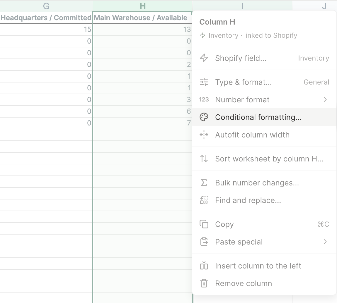
You can also click any cell in the column and choose Column > Conditional formatting… from the menu bar.
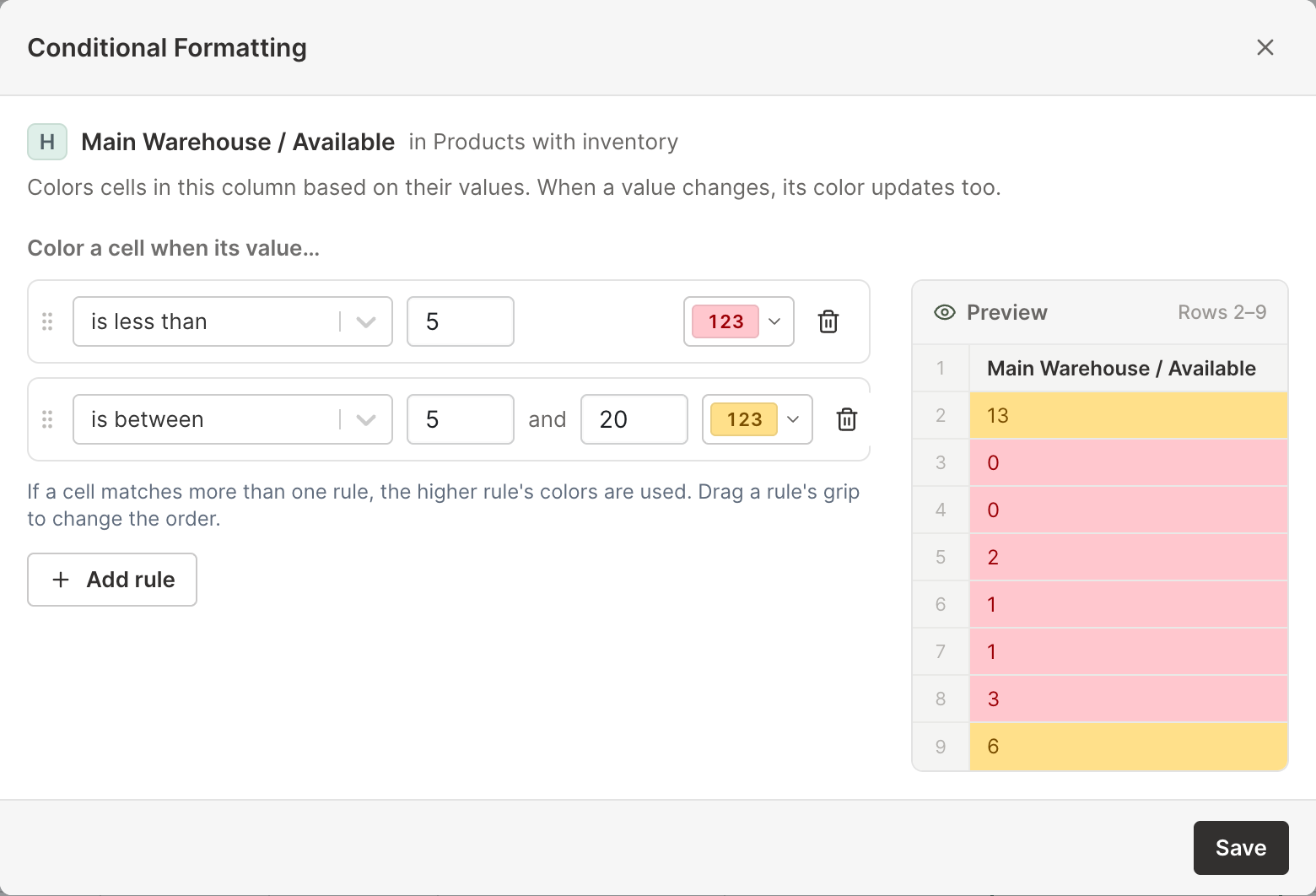
The Conditional Formatting window opens. At the top, it names the column and the worksheet it’s in. Your rules go on the left, and a preview of the column sits on the right.
Note: Adding rules needs permission to edit the worksheet. If the spreadsheet was shared with you with Read only access to this worksheet, Mixtable shows “You don’t have permission to write in this worksheet” instead of opening the window.
Add a rule
- Click Add rule. On a column without rules, you’ll find it in the No rules yet box
- Mixtable adds a rule with a light red fill and dark red text. Each rule reads like a sentence, for example “Color a cell when its value… is less than 5”. Open the rule’s condition menu and choose the condition you want. The next section lists every condition
- Type the value the condition compares against, for example
5. is between and is not between have two boxes. The date conditions, is empty, and is not empty don’t need a value - To change the colors, click the color button at the end of the rule (it shows 123 or Abc in the rule’s colors). See Choose the colors below
- Check the preview on the right to see which cells the rule colors
- Click Save
Save stays grayed out until every rule has its values and something has changed. Once your rules are saved, Mixtable shows “Saved conditional formatting” and colors the column.
Tip: In a number box, type a plain number such as 5, 19.99, or -2.5, without currency symbols, commas, or percent signs. The box turns red if what you typed isn’t a number.
Conditions you can use
The condition menu groups the conditions by the kind of value they check. If most of the column’s values are numbers, Numbers comes first and a new rule starts with is less than. Otherwise Text comes first and a new rule starts with contains.
Numbers
| Condition | Colors a cell when its value |
|---|---|
| is less than | is below your number |
| is at most | is your number or below it |
| is greater than | is above your number |
| is at least | is your number or above it |
| is equal to | is exactly your number |
| is not equal to | is any other number |
| is between | is between your two numbers, including both of them |
| is not between | is below the lower number or above the higher one |
A few things worth knowing:
- Number conditions also read text that looks like a number, such as
$12.50or1,234. Blank cells and text that isn’t a number, such asN/A, never match - You can type the two numbers of is between in either order
- In a spreadsheet, a percentage is a fraction: 30% is the value 0.3. So to color percentages under 30%, use is less than
0.3
Text
| Condition | Colors a cell when its value |
|---|---|
| contains | includes your text anywhere |
| does not contain | doesn’t include your text |
| starts with | begins with your text |
| ends with | ends with your text |
| is exactly | is your text and nothing else |
Upper and lower case don’t matter, so draft also matches DRAFT and Draft. Characters such as * and ? match themselves rather than acting as wildcards. Blank cells never match a text condition. You type the text yourself, even on a dropdown column.
Dates
| Condition | Colors a cell when its value |
|---|---|
| is today | is today’s date |
| is in the last 7 days | is today or one of the 6 days before it |
| is this month | falls in the current month |
| is last month | falls in the previous month |
Date conditions work with the dates Shopify sends, such as an order’s Created At, and with dates you type. They use your computer’s date and time zone, so “today” means today where you are.
Any value
| Condition | Colors a cell when its value |
|---|---|
| is empty | is blank |
| is not empty | has anything in it |
is empty colors a blank cell only when something else in its row has a value, so the empty rows below your data stay plain.
Choose the colors
Each rule sets a fill color, a text color, or both. Click the color button at the end of a rule to open its colors:
- Styles: six ready-made pairs that keep text easy to read: light red fill with dark red text, amber fill with dark amber text, light green fill with dark green text, light blue fill with dark blue text, gray fill with dark gray text, and red text with no fill. Point at a style to see its name
- Fill color: pick a fill, or None to leave the cell’s own fill showing
- Font color: pick a text color, or None to leave the cell’s own text color showing
A rule needs at least one color, so you can’t set both to None. The fill and font colors are the same ones the toolbar’s Fill Color and Font Color buttons offer.
Use more than one rule
A column can have up to 20 rules. Once you reach 20, Add rule is grayed out.
Mixtable checks each cell against the rules from top to bottom and uses the colors of the first rule it matches. As the window puts it: “If a cell matches more than one rule, the higher rule’s colors are used.” A cell never mixes colors from two rules.
To change the order, drag a rule by its grip (the dotted handle at its left end) and drop it above or below another rule.
Order matters when rules overlap. Say you have is less than 5 in red above is less than 20 in amber. A stock level of 3 turns red and 12 turns amber. Swap the two rules and both turn amber, because 3 is less than 20 too.
Check the preview
The preview on the right shows the column’s header and up to eight rows of data (rows 2 to 9), colored the way your rules would color them. It updates as you change the rules, before you save, so you can try a condition and see what it catches. A rule you haven’t finished yet colors nothing.
The preview only shows the first rows. Once you save, the rules cover the whole column. If the column has no values yet, the preview says “This column has no data yet.”
What happens when values change
Rules keep working after you save. Mixtable checks a cell again whenever its value changes, so:
- Colors update when you edit or paste values, and when changes come in from Shopify
- Rows added later, such as new products that come in from Shopify, get colored too
- Everyone who has the spreadsheet open sees the colors as soon as you save
A few things stay the way they are:
- The header row (row 1) is never colored
- A cell you’ve edited but not yet synced to Shopify keeps its light yellow highlight, so pending changes still stand out
- Rule colors sit on top of a cell’s own formatting without replacing it. When a cell stops matching, its own colors show again. The toolbar’s Clear Formatting button doesn’t remove rule colors
Exporting colored worksheets
- Import & Export > Export to Excel keeps your rules. They’re saved in the .xlsx file as Excel conditional formatting, not as fixed colors
- Import & Export > Export to CSV saves values only. A CSV file can’t hold colors, so the rules don’t come along
Edit or remove rules
- Open Conditional formatting… for the column again
- Change a rule’s condition, value, or colors, or drag a rule to a new place. To remove a rule, click the trash can at its end (Delete rule)
- Click Save
To stop coloring a column, delete all of its rules and click Save. If you close the window without saving, Mixtable drops your changes and keeps the rules you had.
What conditional formatting can’t do
- It colors the matching cell only, not the whole row
- Rules set fill and text colors only. They can’t make text bold or italic, change its size, or add borders
- A rule compares each cell with a number or text you type. It can’t compare a cell with another cell or column, or use a formula
- There are no color scales, data bars, top 10 rules, or above average rules, and no rule for duplicate values
- Each column has its own rules. To color another column, open Conditional formatting… for that column and add rules there
To change how values look, such as currency, dates, or bold text, see Format cells and columns.